Date: 24-09-2025

Logistic Regression

Why it matters

Useful for predicting a categorical label from continuous feature data. Classification achieved via probabilities.

Assumptions & Preconditions

Predicting a class from a continuous feature vector
Linear relationship between the features and the log-odds of the class prediction
Absence of multicollinearity — for example, age and no. years work experience should be collapsed together via PCA/otherwise.
Sufficient sample size for minority class (e.g. fraud detection has a low sample size)

How it works (intuition)

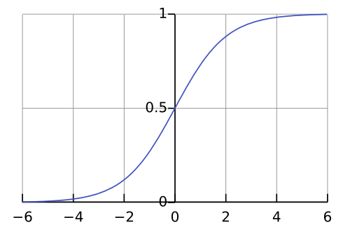
You pass your linear combination of feature vectors $z = β_{0} + β_{1} x_{1} + β_{2} x_{2} + . . . + β_{p} x_{p}$ which lies somewhere in $R$ and map it to $[0, 1]$ to get a probability via $σ (z) = \frac{1}{1 + e^{- z}}$ . Set some threshold; probabilities above are assigned class A, below get class B.
Logistic Curve
Assuming we're predicting $y \in {0, 1}$ , to find $β$ , you look at your data ${x_{i}, y_{i}}_{i = 1}^{m}$ and write down the likelihood function (just rewarding successes and disincentivizing failures as appropriate)

L (β) = \prod_{i = 1}^{m} σ (z_{i})^{y_{i}} (1 - σ (z_{i}))^{1 - y_{i}}

Optimising $L$ is equivalent to optimising the log-likelihood,

L (β) = \sum_{i = 1}^{m} [y_{i} \log (σ (z_{i})) + (1 - y_{i}) \log (1 - σ (z_{i}))]

With some regularisation added to the loss function, this gets messy and the optimal parameters on the data are found numerically. See docs and my 2nd year notes on finding MLEs for details.

Minimal Recipe

from sklearn.linear_model import LogisticRegression
y = df['target_label']
X = df.drop(['target_label'], axis=1)
# >>> scale the dataset, feature engineering... >>>
X_train, X_test, y_train, y_test = train_test_split(X, y)

model = LogisticRegression(c=300) # defaults to L2 regularisation
model.fit(X_train, y_train)

y_pred = model.predict(X_test) # predict class labels
y_prob = (model.predict_proba(X_test)[:, 1] >= 0.5).astype(int) # probablities for both classes and convert to a label

Note: multi-class labelling is easy to achieve. Lots of different implementations (OvR, OvO or softmaxing the multinomial). Requires careful pre-processing.

Pitfalls

Remember:

You need a sufficient sample size — at least 20-30 observations per feature — otherwise you can easily overfit.
By using buckets for classification, a 0.6 and a 0.99 will be given the same label despite wildly different levels of confidence.
- Consider more buckets (e.g. low risk, medium risk, high risk), using the underlying probabilities for maximum interpretability.

Metrics & Checks

When predicting a class label, you can be wrong in two ways:

False positive — predicted true when actually false
False negative — predicted false when actually true

These are measured as follows:

Accuracy: What's the proportion of correctly classified predictions?

Accuracy = \frac{TP + TN}{TP + TN + FP + FN}

Recall: What proportion of the predicted positives were genuine?

Recall = \frac{TP}{TP + FN}

Precision: What fraction of the true positives are we capturing?

Precision = \frac{TP}{TP + FP}

F1-Score: harmonic mean of recall and precision — a single metric to balance the trade-off

F1-Score = 2 \times \frac{Precision \times Recall}{Precision + Recall}

The relevance of these metrics is scenario dependent. For example...

A new cancer screening can't afford a false negative so you'd require a high recall score for your model
When detecting fraud, each investigation is costly so you'd prioritise high precision over recall to avoid wasted resource.

Tools & Workflows

Confusion Matrix: how many TP, FP, TN, FN are there? You have a classification report to tell you and can also visualise

from sklearn.metrics import confusion_matrix, ConfusionMatrixDisplay
mat = confusion_matrix(y_test, y_pred)
ConfusionMatrixDisplay(mat).plot;
print(classification_report(y_test, y_pred))

RoC Curve: it's useful to understand how your FP/FN rates change as you modify the threshold.

The True Positive Rate is defined as

TPR = \frac{TP}{TP+FN} = \frac{True Positives}{All Actual Positives}

The False Positive Rate is defined as

FPR = \frac{FP}{FP+TN} = \frac{False Positives}{All Actual Negatives}

Plot these values against each other as the threshold increases to get an intuition for a good threshold value

from sklearn.metrics import roc_curve, auc
y_probs = model.predict_proba(X_test)[:, 1] # probabilities for the first label only
fpr, tpr, thresholds = roc_curve(y_test, y_probs) # finds
roc_auc = auc(fpr, tpr)

# plot
plt.plot(fpr, tpr) # limit values to [0,1]^2
plt.xlabel('False Positives Rate') 
plt.ylabel('True Positives Rate')

You can then find an optimal index dependent on your situation (fbeta score gives you maximum control). For example

optimal_index = np.argmax(tpr * (1-fpr)) # balance between FP and TP
best_threshold = thresholds[optimal_index]

Dealing with class imbalances: most financial transactions are not fraudulent, creating an imbalanced dataset. If we try and train a model on this dataset directly, the minority class will be predicted poorly. Two standard routes forwards:
1. Move the data around — undersampling, oversampling, SMOTE, SMOTENC. This can introduce unwanted bias so be careful.
2. Change the model — e.g. change class weights to force the model to care more about the minority class.